There are two road crossings (purple bicycle icon in the map below) that are currently have no painted crosswalk or signage: 1) At the edge of Brookfield, crossing Sunset Rd at Marcasite Dr or Copperstone Dr. 2) Crossing Split Log Rd just beyond the end of the sidewalk along Split Log Rd that branches off from the Sunset Rd greenway. This second crossing involves a short segment (~250ft) of walking or riding along Split Log Rd, with good visibility in both directions.

After crossing Split Log Rd, the route enters a new neighborhood (roads do not yet appear on Google Maps as of 2024-08-27) that connects with the Benington neighborhood.

The KML file for this route is available here: brookfield_to_sunset.kml. An interactive Google Map version of the route is displayed below.

If a lead rope solo (LRS) climber could carry a rope for each pitch of a multipitch route, and all gear needed without reusing any, then each pitch could be climbed just once using the "regular" LRS method. Otherwise, for each pitch, the climber must lower, clean gear, untie the lead rope from the anchor, and re-climb or ascend the pitch (see Brent Barghahn's "Redpoint Rope Soloing Revised" for an overview of a modern LRS system). The modified LRS method below could be used to climb each pitch once, reusing the same rope for each pitch, but still requires the climber to carry all anchor and protection gear needed without reusing any.

Method: Like "regular" LRS, the lead rope is fixed to an anchor then passes up through protection and back to the climber through a self-belay device. However, at the anchor, the rope is fixed using a tube device in guide mode (e.g., the Black Diamond ATC Guide) that permits upward progress but blocks during a fall (see diagram below). The anchor end of the rope is tied to a tag line attached to the climber. While climbing, the tag line is extended as needed such that the lead rope remains stationary. At the top of each pitch, the climber disconnects the rope from the self-belay device and pulls the tag line and lead rope from the opposite end, through all of the protection, through the tube device at the anchor, and back up to the climber. This frees the rope for the next pitch where the process is repeated. At the top of the final pitch, the climber rappels and cleans each pitch.

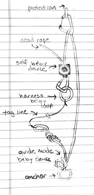
The main benefit of this technique is to climb each pitch without lowering and re-climbing, and still be able to reuse the rope. There are several drawbacks, relative to the "regular" LRS method:

1. Lead climbing is not listed as an application for some tube devices in guide mode (e.g., the Mammut Wall Alpine Belay). The configuration depicted above is further complicated because it's upside down from the usual guide mode, and because the "brake" side is dangling free. The consequences of a lead fall on a tube device in this configuration are unclear.
2. This method requires enough anchor and protection gear for all pitches without reuse, including an extra tube device in guide mode for the anchor of each pitch. And, all gear is left in place until the final descent. A shorter sport route, such as Star Chek (3 pitches, 16 bolts total) might be suitable for this method.
3. The rope may get stuck while pulling the end through the tube device.
4. Due to the previous concern, it's risky to lead more than 1/2 of the rope length.
5. Backfeed prevention widgets may prevent rope retrieval.

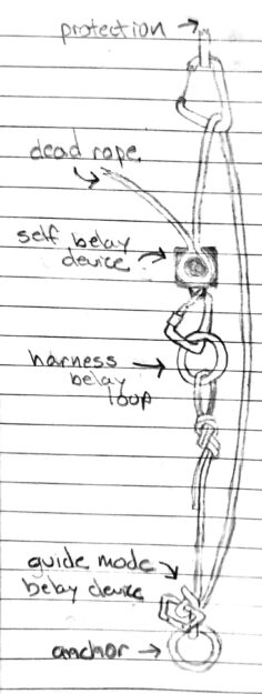
Variation: Instead of tying the lead rope to a tag line, it can be tied directly to the harness. While climbing, both ends of the lead rope move upward. See diagram below. However, there is significant rope friction due to movement through the tube device and protection each time the climber moves upward.

It took about 12 hours in the dehydrator until the oatmeal became brittle. The mango was dry after 8 hours or so.

To rehydrate, I added just enough water to cover the dehydrated oats and mango and simmered the mixture for about 5 minutes, stirring frequently to break up the pieces. The result was pretty similar to my standard steel cut oatmeal preparation (without the dehydration-rehydration step). However, I think a few additional minutes of simmering would have made it better.

Overall, I think this method could work for backpacking, but it's not worth the effort when rolled or "quick cook steel cut" oats can be cooked from scratch in the time needed to rehydrate steel cut oats. However, the mango was excellent and rehydrated very well.

TLDR:

• Begin with N of 10, increase by 10 until p < 0.05 or max N reached.
• This design has inflated type-I error.
• Lower p-value threshold needed to ensure specified type-I error rate.
• The number of interim analyses and max N affect the type-I error rate.
• Threshold can be identified using simulation.

A recent Facebook post to a statistician group highlighted a basic science article (in a Nature journal: https://www.nature.com/articles/s41467-017-02765-w#Sec10) that used a 'foolproof' study design: "we continuously increased the number of animals until statistical significance was reached to support our conclusions." Many of the statisticians in the group were exasperated! The group was rightly critical of the authors' brazen approach, but also due to the resulting inflated type-I error rate. However, as the following code demonstrates, this approach needs only a simple modification to become a valid (i.e., by preserving the specified type-I error rate) adaptive trial design.

For simplicity (and completeness), consider a block-randomized two sample comparison using a t-test. Then, begin with a sample size of 10 in each group and increase by 10 until p < 0.05 or until a maximum sample size is reached.

The code chunk below simulates this study design. This process was repeated many times under the null hypothesis (no difference in mean outcome) and the test results used to estimate the actual type-I error rate, as well as the median (IQR) total sample size. When the maximum sample size is 100 per group, the type-I error rate is about 19% and the median (IQR) sample size is 100 (100, 100) per group. If the sample size increment is 5 instead of 10, the type-I error rate is about 24%. When the maximum sample size is 1000 per group, type-I error rate is about 37% and the median (IQR) sample size is 1000 (200, 1000) per group. Thus, smaller sample size increment (more frequent interim analysis) and larger maximum sample size both result in a larger type-I error rate.

19%, 24%, and 37% are obviously unacceptably large type-I error rates. However, the specified type-I error rate (usually 5%) can be achieved by modifying the p-value threshold. The final code chunk below demonstrates that, by using a p-value threshold of 0.01 (found by guess-and-check), maximum sample size of 100, and sample size increment at 10, the type-I error rate is about 5%. This also has the effect that the maximum sample size is reached in about 95% of simulated studies, under the null.

## consider a two sample problem tested using t-test; start with 'n'
## in each group, increase by 'n' until p< 'alp' or maximum sample size
## 'nmx' reached

## simulate data 
## n   - sample size increment per group
## eff - effect size (difference in means; eff=0 is null hypothesis)
sim <- function(n=10, eff=0)
  data.frame(y1=rnorm(n), y2=rnorm(n, mean=eff))

## compute test
## dat - data from sim() function
## alp - significance threshold
tst <- function(dat, alp=0.05) 
  t.test(dat$y1, dat$y2)$p.value < alp

## apply the 10+10 algorithm
## n   - sample size in each of two groups
## eff - effect size (difference in means; eff=0 is null hypothesis)
## alp - significance threshold
## nmx - maximum sample size in each of two groups
alg <- function(n=10, eff=0, alp=0.05, nmx=1000) {
  dat <- sim(n,eff)
  rej <- tst(dat, alp)
  while(nrow(dat) < nmx && !rej) {
    dat <- rbind(dat, sim(n,eff))
    rej <- tst(dat, alp)
  }
  list(n = 2*nrow(dat), rej = rej)
}

## calculate overall type-I error by simulating study under null
## repeat procedure 5k times under null with nmx=100
out <- replicate(5000, alg(nmx=100), simplify=FALSE)
## estimate type-I error; fraction of times null rejected
mean(sapply(out, `[[`, 'rej'))
## distribution of total sample size (pairs)
quantile(sapply(out, `[[`, 'n')/2, probs=c(0.25, 0.50, 0.75))

## calculate overall type-I error by simulating study under null
## repeat procedure 5k times under null with nmx=100, and interim
## analysis at every 5 samples
out <- replicate(5000, alg(n=5, nmx=100), simplify=FALSE)
## estimate type-I error; fraction of times null rejected
mean(sapply(out, `[[`, 'rej'))
## distribution of total sample size (pairs)
quantile(sapply(out, `[[`, 'n')/2, probs=c(0.25, 0.50, 0.75))

## calculate overall type-I error by simulating study under null
## repeat procedure 5k times under null with nmx=1000
out <- replicate(5000, alg(nmx=1000), simplify=FALSE)
## estimate type-I error; fraction of times null rejected
mean(sapply(out, `[[`, 'rej'))
## distribution of total sample size (pairs)
quantile(sapply(out, `[[`, 'n')/2, probs=c(0.25, 0.50, 0.75))

## can the type-I error be fixed by adjusting threshold?
## repeat procedure 
out <- replicate(5000, alg(alp=0.01, nmx=100), simplify=FALSE)
## estimate type-I error
mean(sapply(out, `[[`, 'rej'))
## distribution of total sample size (pairs)
table(sapply(out, `[[`, 'n'))

## Simulate Bayesian single-arm adaptive trial
## Allow early termination due to futility or efficacy
## Binary outcome
## Beta-binomial:
##   p   ~ beta(a, b)
##   x_i ~ binomial(p)  i = 1..n
##   p|x ~ beta(a + sum(x), b + n - sum(x))
## Efficacy at interim t if Pr(p > p_0 | x_{(t)}) > \gamma_e
## Futility at interim t if Pr(p > p_0 | x_{(t_max)}) < \gamma_f
## https://www.ncbi.nlm.nih.gov/pmc/articles/PMC4247348/

library('rmutil') ## for betabinom
## Simulate entire trial
## ptru - true probability of outcome (p)
## pref - reference probability of outcome (p_0)
## nint - sample sizes at which to conduct interim analyses
## efft - efficacy threshold
## futt - futility threshold
## apri - prior beta parameter \alpha
## bpri - prior beta parameter \beta
simtrial <- function(
  ptru = 0.15,
  pref = 0.15,
  nint = c(10, 13, 16, 19),
  efft = 0.95,
  futt = 0.05,
  apri = 1,
  bpri = 1) {
  
  ## determine minimum number of 'successes' necessary to 
  ## conclude efficacy if study continues to maximum 
  ## sample size
  nmax <- max(nint)
  post <- sapply(0:nmax, function(nevt)
    1-pbeta(pref, apri + nevt, bpri + nmax - nevt))
  nsuc <- min(which(post > efft)-1)
  
  
  ## simulate samples
  samp <- rbinom(n = nmax, size = 1, prob = ptru)
  
  ## simulate interim analyses
  intr <- lapply(nint, function(ncur) {
    
    ## compute number of current events
    ecur <- sum(samp[1:ncur])
    
    ## compute posterior beta parameters
    abb <- apri + ecur
    bbb <- bpri + ncur - ecur
    sbb <- abb + bbb
    mbb <- abb/(abb+bbb)
    
    ## compute efficacy Pr(p > p_0 | x_{(t)})
    effp <- 1-pbeta(pref, abb, bbb)
    
    ## return for efficacy
    if(effp > efft)
      return(list(action='stop',
                  reason='efficacy',
                  n = ncur))
    
    ## number of events necessary in remainder of 
    ## study to conclude efficacy
    erem <- nsuc-ecur

    ## compute success probability Pr(p > p_0 | x_{(t_max)})
    if(erem > nmax-ncur) { ## not enough possible events
      sucp <- 0
    } else { ## not yet met efficacy threshold
      sucp <- 1-pbetabinom(q = erem-1, 
        size = nmax-ncur, m = mbb, s = sbb)
    }
    
    if(sucp < futt)
      return(list(action='stop',
                  reason='futility',
                  n = ncur))
    
    return(list(action='continue',
                reason='',
                n = ncur))
  })
  
  stpi <- match('stop', sapply(intr, `[[`, 'action'))
  return(intr[[stpi]])
}


## Simulate study with max sample size of 200 where true 
## probability is identical to reference (i.e., the null
## hypothesis is true). This type of simulation helps us 
## determine the overall type-I error rate.
nint <- c(40,80,120,160,200)
nmax <- max(nint)
res <- do.call(rbind, lapply(1:10000, 
  function(t) as.data.frame(simtrial(ptru = 0.72, 
                                     pref = 0.72,
                                     nint = nint,
                                     efft = 0.975,
                                     futt = 0.20))))

## Prob. early termination (PET) due to Futility
mean(res$reason == 'futility' & res$n < nmax)
## PET Efficacy
mean(res$reason == 'efficacy' & res$n < nmax)
## Pr(conclude efficacy) 'type-I error rate'
mean(res$reason == 'efficacy')
## average and sd sample size
mean(res$n); sd(res$n)
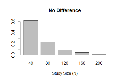
barplot(prop.table(table(res$n)),
        xlab='Study Size (N)',
        main="No Difference")

## Simulate study where true probability is greater than
## reference (i.e., an alternative hypothesis). This type
## of simulation helps us determine the study power.
res <- do.call(rbind, lapply(1:10000, 
  function(t) as.data.frame(simtrial(ptru = 0.82, 
                                     pref = 0.72,
                                     nint = nint,
                                     efft = 0.975,
                                     futt = 0.20))))

## Prob. early termination (PET) due to Futility
mean(res$reason == 'futility' & res$n < nmax)
## PET Efficacy
mean(res$reason == 'efficacy' & res$n < nmax)
## Pr(conclude efficacy) 'power'
mean(res$reason == 'efficacy')
## average and sd sample size
mean(res$n); sd(res$n)
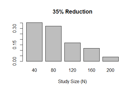
barplot(prop.table(table(res$n)),
        xlab='Study Size (N)',
        main="35% Reduction")

## Metropolis sampling
## x    - current value of Markov chain (numeric vector)
## targ - target log density function
## prop - function with prototype function(x, ...) that generates 
##   a proposal value from a symmetric proposal distribution
library('mvtnorm')
prop_mvnorm <- function(x, ...)
  drop(rmvnorm(1, mean=x, ...))
metropolis <- function(x, targ, prop=prop_mvnorm, ...) {
  xnew <- prop(x)
  lrat <- targ(xnew, ...) - targ(x, ...)
  if(log(runif(1)) < lrat)
    x <- xnew
  return(x)
}

## Metropolis-in-Gibbs sampling
## x    - current value of Markov chain (numeric vector)
## targ - target log density function
## ...  - arguments passed to 'targ'
gibbs <- function(x, targ, ...) {
  for(i in 1:length(x)) {
    ## define full conditional
    targ1 <- function(x1, ...) {
      x[i] <- x1
      targ(x, ...)
    }
    ## sample using Metropolis algorithm
    x[i] <- metropolis(x[i], targ1, ...)
  }
  return(x)
}

The following code produces the figure below to illustrate the two methods using a 'dumbell' distribution (cf. R package 'ks' vignette).

### The code below illustrates the use of the functions above 

## target 'dumbell' density (c.f., R package 'ks' vignette)
library('ks')
mus <- rbind(c(-2,2), c(0,0), c(2,-2))
sigmas <- rbind(diag(2), matrix(c(0.8, -0.72, -0.72, 0.8), nrow=2), diag(2)) 
cwt <- 3/11
props <- c((1-cwt)/2, cwt, (1-cwt)/2)
targ_test <- function(x, ...)
  log(dmvnorm.mixt(x, mus=mus, Sigmas=sigmas, props=props))

## plot contours of target 'dumbell' density
set.seed(42)
par(mfrow=c(1,2))
plotmixt(mus=mus, Sigmas=sigmas, props=props,
         xlim=c(-4,4), ylim=c(-4,4),
         xlab=expression(x[1]),
         ylab=expression(x[2]),
         main="Metropolis-in-Gibbs")

## initialize and sample using Metropolis-in-Gibbs
xcur <- gibbs(c(0,0), targ_test, sigma=vcov_test)
for(j in 1:2000) {
  xcur <- gibbs(xcur, targ_test, sigma=vcov_test)
  points(xcur[1], xcur[2], pch=20, col='#00000055')
}

## plot contours of target 'dumbell' density
plotmixt(mus=mus, Sigmas=sigmas, props=props,
         xlim=c(-4,4), ylim=c(-4,4),
         xlab=expression(x[1]),
         ylab=expression(x[2]),
         main="Metropolis")

## initialize and sample using Metropolis
xcur <- metropolis(c(0,0), targ_test, sigma=vcov_test)
for(j in 1:2000) {
  xcur <- metropolis(xcur, targ_test, sigma=vcov_test)
  points(xcur[1], xcur[2], pch=20, col='#00000055')
}

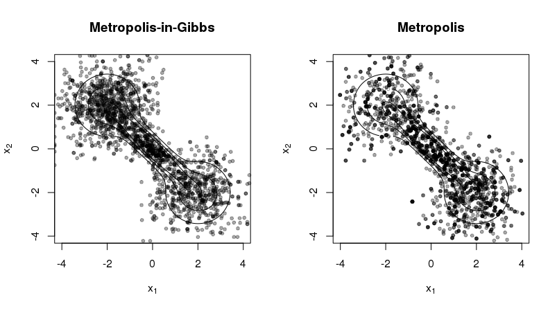
The figure illustrates two contrasting properties of the two methods:

1. Metropolis-in-Gibbs samples can get 'stuck' in certain regions of the support, especially when there are multiple modes and/or significant correlation among the random variables. This is not as much a problem for Metropolis sampling.
2. Metropolis sampling can produce fewer unique samples due to the poor approximation of the proposal density to the target density. This occurs more often for high-dimensional target densities.